Randomized experiments

class: center, middle, inverse, title-slide

# Randomized experiments
## What If: Chapter 2
### Elena Dudukina
### 2020-10-18

---

Only one of the two counterfactual outcomes is known: the one corresponding to the treatment level actually received

```
## # A tibble: 20 x 5
##    greek          A Y_obs  Y_a0  Y_a1
##    <chr>      <dbl> <dbl> <dbl> <dbl>
##  1 Rheia          0     0     0    NA
##  2 Kronos         0     1     1    NA
##  3 Demeter        0     0     0    NA
##  4 Hades          0     0     0    NA
##  5 Hestia         1     0    NA     0
##  6 Poseidon       1     0    NA     0
##  7 Hera           1     0    NA     0
##  8 Zeus           1     1    NA     1
##  9 Artemis        0     1     1    NA
## 10 Apollo         0     1     1    NA
## 11 Leto           0     0     0    NA
## 12 Ares           1     1    NA     1
## 13 Athena         1     1    NA     1
## 14 Hephaestus     1     1    NA     1
## 15 Aphrodite      1     1    NA     1
## 16 Cyclope        1     1    NA     1
## 17 Persephone     1     1    NA     1
## 18 Hermes         1     0    NA     0
## 19 Hebe           1     0    NA     0
## 20 Dionysus       1     0    NA     0
```
---

# Randomized experiments
- Randomization ensures that the missing values on potential outcomes (PO) occurred by chance
- Effect measures can be consistently estimated
---
# Hypothetical randomized experiment

![:scale 40%](fig 1.1.png)
- Flipping **not** a fair coin
    - if tails → assign treatment A=1/membership in a "white" group
    - otherwise → treatment A=0/membership in a "grey" group
    - probability of tossing tails is 0.6
- Associational risk ratio: `$Pr[Y=1|A=1]$` / `$Pr[Y=1|A=0]$` = 0.3/0.6 = 0.5
- Assumptions: no loss to follow-up, full adherence to the assigned treatment over the duration of the study, a single version of treatment, and double blind assignment
- Had we assigned the reverse treatment levels at random to this population, the association would be the same
---
# Exchangeability
- When group membership is randomized, which particular group gets the treatment is irrelevant for the value of `$Pr[Y=1|A=1]$` (conditional probability of the outcome given the exposure level)
--

- The probability of the potential outcome `$Y^a$` is the same under A=1 and A=0
    - `$Pr[Y^{a}=1|A=1]$` = `$Pr[Y^{a}=1|A=0]$`, then 
    - `$Pr[Y^{a}=1|A=1]$` = `$Pr[Y^{a}=1|A=0]$` = `$Pr[Y^{a}=1]$` (in RCT)
--

- `$Y^{a}\perp\perp\ A$` for all `$a$`
- For the binary treatment variable scenario:
    - `$Y^{a}\perp\perp\ A=1$`
    - `$Y^{a}\perp\perp\ A=0$`
--
    
- The actual treatment level A **does not** predict PO `$Y^a$`
    - Knowing the actual received treatment level does not tell you anything about the probability of the PO outcome in that group
---
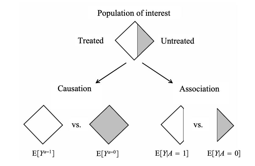
# In an ideal randomized experiment the association is causation
Under exchangeability:
- `$Pr[Y^{a}=1]$` = `$Pr[Y^{a}=1|A=a]$`
--
- `$Pr[Y^{a=1}=1]$` = `$Pr[Y^{a=1}=1|A=1]$` 
- `$Pr[Y^{a=0}=1]$` = `$Pr[Y^{a=0}=1|A=0]$` 
---
# Exchangeability is about PO outcome independence of actual treatment
- Exchangeability: `$Y^{a}\perp\perp\ A$`
- Conditional independence of two observed variables: `$Y\perp\perp\ A$`

---
# Hypothetical exchangeability assumption check
- In reality, exchangeability is untestable assumption
- To explore the concept of exchangeability, we go back to table 1.1, where we have hypothetical data on **both** potential outcomes under A=1 and under A=0
---
# Greek gods, their actual treatment level and POs under actual and counterfactual levels of treatment

```
## # A tibble: 20 x 4
##    greek          A  Y_a0  Y_a1
##    <chr>      <dbl> <dbl> <dbl>
##  1 Rheia          0     0     1
##  2 Kronos         0     1     0
##  3 Demeter        0     0     0
##  4 Hades          0     0     0
##  5 Hestia         1     0     0
##  6 Poseidon       1     1     0
##  7 Hera           1     0     0
##  8 Zeus           1     0     1
##  9 Artemis        0     1     1
## 10 Apollo         0     1     0
## 11 Leto           0     0     1
## 12 Ares           1     1     1
## 13 Athena         1     1     1
## 14 Hephaestus     1     0     1
## 15 Aphrodite      1     0     1
## 16 Cyclope        1     0     1
## 17 Persephone     1     1     1
## 18 Hermes         1     1     0
## 19 Hebe           1     1     0
## 20 Dionysus       1     1     0
```
---
# Explore exchangeability assumption among greek gods
- `$Y^{a=0}$`
    - Had the treated and untreated gods were exchangeable, `$Y^{a}\perp\perp\ A$` and `$Pr[Y^{a}=1|A=1]$` = `$Pr[Y^{a}=1|A=0]$`
    - Is `$Y^{a}\perp\perp\ A$` for `$a=0$` → `$Pr[Y^{a=0}=1|A=0]$` = `$Pr[Y^{a=0}=1|A=1]$`?

```r
greek_gods_potential_outcomes %>% 
  group_by(A) %>% 
  count(Y_a0) %>% 
  mutate(
    denominator = sum(n),
    pr_of_Y_a0 = round(n / denominator, 2)
  ) %>% 
  filter(Y_a0 == 1)
```

```
## # A tibble: 2 x 5
## # Groups:   A [2]
##       A  Y_a0     n denominator pr_of_Y_a0
##   <dbl> <dbl> <int>       <int>      <dbl>
## 1     0     1     3           7       0.43
## 2     1     1     7          13       0.54
```
---
- `$Pr[Y^{a=0}=1|A=0]$` = 0.43 and `$Pr[Y^{a=0}=1|A=1]$` = 0.54, then
  - `$Pr[Y^{a=0}=1|A=0]$` < `$Pr[Y^{a=0}=1|A=1]$` 
  - Under consistency: `$Pr[Y^{a=0}=1|A=0]$` = `$Pr[Y=1|A=0]$`
  - In words, treated individuals had they been untreated (A=0) had a higher probability of dying
  - Exchangeability does not hold for the greek gods
 
---
# Explore exchangeability assumption among greek gods
- `$Y^{a=1}$`
    - Is `$Y^{a}\perp\perp\ A$` for `$a=1$` → `$Pr[Y^{a=1}=1|A=0]$` = `$Pr[Y^{a=1}=1|A=1]$`?

```r
greek_gods_potential_outcomes %>% 
  group_by(A) %>% 
  count(Y_a1) %>% 
  mutate(
    denominator = sum(n),
    pr_of_Y_a1 = round(n / denominator, 2)
  ) %>% 
  filter(Y_a1 == 1)
```

```
## # A tibble: 2 x 5
## # Groups:   A [2]
##       A  Y_a1     n denominator pr_of_Y_a1
##   <dbl> <dbl> <int>       <int>      <dbl>
## 1     0     1     3           7       0.43
## 2     1     1     7          13       0.54
```
---
  - `$Pr[Y^{a=1}=1|A=0]$` = 0.43 and `$Pr[Y^{a=1}=1|A=1]$` = 0.54, then
  - `$Pr[Y^{a=1}=1|A=0]$` < `$Pr[Y^{a=1}=1|A=1]$`
  - Under consistency: `$Pr[Y^{a=1}=1|A=1]$` = `$Pr[Y=1|A=1]$`
    - In words, actually treated individuals had a higher probability of dying 
      than untreated had they been treated (A=1)
    - Exchangeability does not hold for the greek gods
    - Knowing the actual received treatment level tells us something about the probability of the PO → being treated means having a higher probability of potential death
      
---
# Marginal randomization vs. conditional randomization
- Marginal randomization (RCT): unconditional assignment of treatment probability

- Introducing prognostic factor L

```
## # A tibble: 20 x 6
##    greek          L     A Y_obs  Y_a0  Y_a1
##    <chr>      <dbl> <dbl> <dbl> <dbl> <dbl>
##  1 Rheia          0     0     0     0    NA
##  2 Kronos         0     0     1     1    NA
##  3 Demeter        0     0     0     0    NA
##  4 Hades          0     0     0     0    NA
##  5 Hestia         0     1     0    NA     0
##  6 Poseidon       0     1     0    NA     0
##  7 Hera           0     1     0    NA     0
##  8 Zeus           0     1     1    NA     1
##  9 Artemis        1     0     1     1    NA
## 10 Apollo         1     0     1     1    NA
## 11 Leto           1     0     0     0    NA
## 12 Ares           1     1     1    NA     1
## 13 Athena         1     1     1    NA     1
## 14 Hephaestus     1     1     1    NA     1
## 15 Aphrodite      1     1     1    NA     1
## 16 Cyclope        1     1     1    NA     1
## 17 Persephone     1     1     1    NA     1
## 18 Hermes         1     1     0    NA     0
## 19 Hebe           1     1     0    NA     0
## 20 Dionysus       1     1     0    NA     0
```
---
# Conditional randomization
- Assigning the probability of treatment based on the value of prognostic factor L
- Conditional exchangeability: `$Y^{a}\perp\perp\ A|L$` for all `$a$` and all `$l$` (A and L being variables and `$a$` and `$l$` being values of these variables)
  - Conditional exchangeability given L guarantees the exchangeability within the levels of L
---
# Risk ratio in a conditionally randomized study (observational study)
  - Associations risk ratio

```r
# broke
greek_gods_condrand %>% 
  group_by(A) %>% 
  count(Y_obs) %>% 
  mutate(
    denominator = sum(n),
    risk = round(n/sum(n), digits = 2)
  ) %>% 
  filter(Y_obs == 1)
```

```
## # A tibble: 2 x 5
## # Groups:   A [2]
##       A Y_obs     n denominator  risk
##   <dbl> <dbl> <int>       <int> <dbl>
## 1     0     1     3           7  0.43
## 2     1     1     7          13  0.54
```

```r
0.54/0.43 
```

```
## [1] 1.255814
```
---

```r
# woke
greek_gods_condrand %>% 
  glm(formula = Y_obs ~ A, family = binomial(link = "log")) %>% 
  broom::tidy(exponentiate = T) %>% 
  filter(term == "A") %>% 
  select(term, estimate)
```

```
## # A tibble: 1 x 2
##   term  estimate
##   <chr>    <dbl>
## 1 A         1.26
```
---
# Risk ratio in a conditionally randomized study (e.g., observational study)
- L-stratum specific causal risk ratios 
    1. `$\frac{Pr[Y^{a=1}=1|L=1]}{Pr[Y^{a=0}=1|L=1]}$`
--

2. `$\frac{Pr[Y^{a=1}=1|L=0]}{Pr[Y^{a=0}=1|L=0]}$`
--

- Average causal effect in the entire population:
    - `$\frac{Pr[Y^{a=1}=1]}{Pr[Y^{a=0}=1]}$`
---
# Standardization
- `$\frac{Pr[Y^{a=1}=1|L=1]}{Pr[Y^{a=0}=1|L=1]}$` 
    - under conditional exchangeability = `$\frac{Pr[Y^{a=1}=1|L=1, A=1]}{Pr[Y^{a=0}=1|L=1, A=0]}$`
    - under consistency = `$\frac{Pr[Y=1|L=1, A=1]}{Pr[Y=1|L=1, A=0]}$`
--

- Same for the stratum L=0
    - `$\frac{Pr[Y^{a=1}=1|L=0]}{Pr[Y^{a=0}=1|L=0]}$` = `$\frac{Pr[Y=1|L=0, A=1]}{Pr[Y=1|L=0, A=0]}$`
---
Strata L=0

```r
greek_gods_condrand %>% 
  filter(L == 0) %>% 
  group_by(A) %>% 
  count(Y_obs) %>% 
  mutate(
    denominator = sum(n),
    risk = round(n/sum(n), digits = 2)
  ) %>% 
  filter(Y_obs == 1)
```

```
## # A tibble: 2 x 5
## # Groups:   A [2]
##       A Y_obs     n denominator  risk
##   <dbl> <dbl> <int>       <int> <dbl>
## 1     0     1     1           4  0.25
## 2     1     1     1           4  0.25
```
---
Strata L=1

```r
greek_gods_condrand %>% 
  filter(L == 1) %>% 
  group_by(A) %>% 
  count(Y_obs) %>% 
  mutate(
    denominator = sum(n),
    risk = round(n/sum(n), digits = 2)
  ) %>% 
  filter(Y_obs == 1)
```

```
## # A tibble: 2 x 5
## # Groups:   A [2]
##       A Y_obs     n denominator  risk
##   <dbl> <dbl> <int>       <int> <dbl>
## 1     0     1     2           3  0.67
## 2     1     1     6           9  0.67
```

---
# Standardiazation
Average causal effect for the whole population:
- Weighted average of the effects in L=1 and L=0
- Weights are proportional to the size of L-strata

```r
mean(greek_gods_condrand$L)
```

```
## [1] 0.6
```

`$\frac{Pr[Y^{a=1}=1]}{Pr[Y^{a=0}=1]}$` 
- = `$\frac{\Sigma_lPr[Y^{a=1}=1|L, A=1]*Pr(L)}{\Sigma_lPr[Y^{a=0}=1|L, A=0]*Pr(L)}$` (under conditional exchangeability)
- = `$\frac{\Sigma_lPr[Y=1|L, A=1]*Pr(L)}{\Sigma_lPr[Y=1|L, A=0]*Pr(L)}$` for all `$L=l$` (under consistency)
- = `$\frac{Pr[Y=1|L=0, A=1]*Pr(L=0) + Pr[Y=1|L=1, A=1]*Pr(L=1)}{Pr[Y=1|L=0, A=0]*Pr(L=0) + Pr[Y=1|L=1, A=0]*Pr(L=1)}$`
- = `$\frac{0.25 * 0.4 + 0.67 * 0.6}{0.25 * 0.4 + 0.67 * 0.6}$`
- = `$\frac{0.502}{0.502}$`
- = 1.0

Standardization formula:
`$Pr(Y^a=1)=\Sigma_lPr(Y=1|A=a, L=l)*Pr(L=l)$`
---
# Inverse probability weighting

```r
pr_a <- glm(data = greek_gods_condrand, formula = A~1, family = binomial("logit"))
pr_a_l <- glm(data = greek_gods_condrand, formula = A~L, family = binomial("logit"))

greek_gods_condrand %<>% mutate(
  p_a = predict(object = pr_a, type = "response"),
  p_a_l = predict(object = pr_a_l, type = "response"),
  # average treatment effect
  iptw = if_else(A==1, 1/p_a_l, 1/(1-p_a_l)), # unstabilized weights
  sw_iptw = if_else(A==1, p_a/p_a_l, (1-p_a)/(1-p_a_l)) # stabilized weights
)
```
---

```r
greek_gods_condrand %>% 
  select(iptw, sw_iptw) %>% 
  skimr::skim()
```

Table: Data summary

|                         |           |
|:------------------------|:----------|
|Name                     |Piped data |
|Number of rows           |20         |
|Number of columns        |2          |
|_______________________  |           |
|Column type frequency:   |           |
|numeric                  |2          |
|________________________ |           |
|Group variables          |None       |

**Variable type: numeric**

|skim_variable | n_missing| complete_rate| mean|   sd|   p0|  p25|  p50| p75| p100|hist  |
|:-------------|---------:|-------------:|----:|----:|----:|----:|----:|---:|----:|:-----|
|iptw          |         0|             1|    2| 0.92| 1.33| 1.33| 2.00| 2.0|  4.0|▇▇▁▁▂ |
|sw_iptw       |         0|             1|    1| 0.27| 0.70| 0.87| 0.87| 1.3|  1.4|▃▇▁▁▆ |
---
Figure 2.3

```r
greek_gods_condrand %>% 
  distinct(A, Y_obs, L, iptw, sw_iptw)
```

```
## # A tibble: 8 x 5
##       L     A Y_obs  iptw sw_iptw
##   <dbl> <dbl> <dbl> <dbl>   <dbl>
## 1     0     0     0  2.00   0.7  
## 2     0     0     1  2.00   0.7  
## 3     0     1     0  2.     1.30 
## 4     0     1     1  2.     1.30 
## 5     1     0     1  4.00   1.40 
## 6     1     0     0  4.00   1.40 
## 7     1     1     1  1.33   0.867
## 8     1     1     0  1.33   0.867
```
---

```r
glm(data = greek_gods_condrand, formula = Y_obs~A, family = binomial("log"), weights = iptw) %>% 
  broom::tidy(exponentiate = T) %>% 
  filter(term == "A") %>% 
  select(term, estimate)
```

```
## Warning in eval(family$initialize): non-integer #successes in a binomial glm!
```

```
## # A tibble: 1 x 2
##   term  estimate
##   <chr>    <dbl>
## 1 A         1.00
```

```r
glm(data = greek_gods_condrand, formula = Y_obs~A, family = binomial("log"), weights = sw_iptw) %>% 
  broom::tidy(exponentiate = T) %>% 
  filter(term == "A") %>% 
  select(term, estimate)
```

```
## Warning in eval(family$initialize): non-integer #successes in a binomial glm!
```

```
## # A tibble: 1 x 2
##   term  estimate
##   <chr>    <dbl>
## 1 A         1.00
```
---

```r
# crude 2x2 table
greek_gods_condrand  %>% 
  group_by(A) %>% 
  count(Y_obs) %>% 
  mutate(
    denominator = sum(n)
  ) %>% 
  filter(Y_obs == 1)
```

```
## # A tibble: 2 x 4
## # Groups:   A [2]
##       A Y_obs     n denominator
##   <dbl> <dbl> <int>       <int>
## 1     0     1     3           7
## 2     1     1     7          13
```
---

```r
# unstabilized weights doubled the size of the population
greek_gods_condrand  %>% 
  group_by(A) %>% 
  count(Y_obs, wt = iptw) %>% 
  mutate(
    denominator = sum(n)
  ) %>%
  filter(Y_obs == 1)
```

```
## # A tibble: 2 x 4
## # Groups:   A [2]
##       A Y_obs     n denominator
##   <dbl> <dbl> <dbl>       <dbl>
## 1     0     1  10.0        20.0
## 2     1     1  10.         20.
```
---

```r
# stabilized weights kept the original size of the population
greek_gods_condrand  %>% 
  group_by(A) %>% 
  count(Y_obs, wt = sw_iptw) %>% 
  mutate(
    denominator = sum(n)
  ) %>%
  filter(Y_obs == 1)
```

```
## # A tibble: 2 x 4
## # Groups:   A [2]
##       A Y_obs     n denominator
##   <dbl> <dbl> <dbl>       <dbl>
## 1     0     1  3.50        7.00
## 2     1     1  6.5        13.
```